Excel Assignment Practice 05

Excel Assignment Practice 05: हिंदी में जिसमें Conditional Formatting, Fill Series, Growth Series, Date Series और Custom List के आसान उदाहरण दिए गए हैं। इस प्रैक्टिकल #Excel Assignment में छात्रों के लिए Step by Step समाधान, टेबल फॉर्मेट और जरूरी Formatting Exercises शामिल हैं। Beginners और Computer Course Students आसानी से #Excel सीख सकते हैं। यह #Assignment Spreadsheet Skills को बेहतर बनाने के लिए बेहद उपयोगी है और स्कूल, कॉलेज तथा कंप्यूटर क्लास प्रैक्टिस के लिए एक शानदार गाइड साबित होगा।

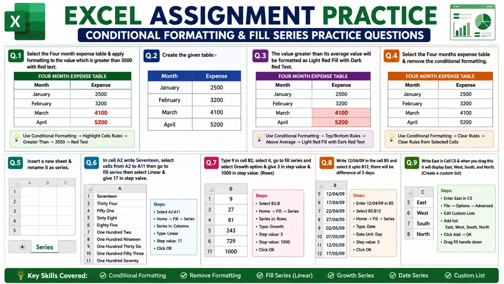
Excel Assignment Practice 05: आसान स्टेप्स के साथ सीखें पूरी Formatting

Q.1- Select the Four Month Expense Table & Apply Formatting to the Value Greater Than 3500 with Red Text

Steps:

1. Select the Four Month Expense Table.
2. Go to the Home tab.
3. Click on Conditional Formatting.
4. Select Highlight Cells Rules.
5. Click on Greater Than.
6. Type 3500 in the box.
7. Choose Red Text formatting.
8. Click OK.

Q.2- Create the Given Table

Month	Expense
January	2500
February	3200
March	4100
April	5200

Q.3- Format the Value Greater Than Its Average Value as Light Red Fill with Dark Red Text

Steps:

1. Select the table values.
2. Go to Home → Conditional Formatting.
3. Click on Top/Bottom Rules.
4. Select Above Average.
5. Choose Light Red Fill with Dark Red Text.
6. Click OK.

Q.4- Select the Four Months Expense Table & Remove the Conditional Formatting

Steps:

1. Select the Expense Table.
2. Go to Home → Conditional Formatting.
3. Click on Clear Rules.
4. Select Clear Rules from Selected Cells.

Q.5- Insert a New Sheet & Rename It as “Series”

Steps:

1. Click on the + (New Sheet) button.
2. A new worksheet will open.
3. Right-click on the sheet name.
4. Select Rename.
5. Type Series and press Enter.

Q.6- In Cell A2 Write “Seventeen”, Select Cells A2 to A11, Then Use Fill Series

Steps:

1. Type Seventeen in cell A2.
2. Select cells from A2 to A11.
3. Go to Home → Fill → Series.
4. Select:
   • Series in: Columns
   • Type: Linear
5. Enter 17 in Step Value.
6. Click OK.

Q.7- Type 9 in Cell B2 & Use Growth Series

Steps:

1. Type 9 in cell B2.
2. Select the required cells in column B.
3. Go to Home → Fill → Series.
4. Select:
   • Series in: Rows
   • Type: Growth
5. Enter:
   • Step Value = 3
   • Stop Value = 1000
6. Click OK.

Q.8- Write 12/04/09 in Cell B5 & Create Date Series with Difference of 5 Days

Steps:

1. Type 12/04/09 in cell B5.
2. Select cells from B5 to B12.
3. Go to Home → Fill → Series.
4. Select:
   • Type = Date
   • Date Unit = Day
5. Enter 5 in Step Value.
6. Click OK.

Q.9- Write East in Cell C5 & Create Custom List

Steps:

1. Type East in cell C5.
2. Go to File → Options → Advanced.
3. Click on Edit Custom Lists.
4. Create the list:
   • East
   • West
   • South
   • North
5. Click Add → OK.
6. Now drag the fill handle from C5 downward.
7. Excel will display: East, West, South, North.