Excel Assignment Practical 03: सीखें Row Insert, Merge Cell, Currency Format, Accounting Format, Table Style Medium 14, Name Box और Date Formatting का सबसे आसान तरीका। यह Step By Step #Practical Guide विद्यार्थियों, कंप्यूटर कोर्स स्टूडेंट्स और Beginners के लिए तैयार की गई है। अगर आप #Excel #Assignment को सही और Professional तरीके से करना चाहते हैं, तो यह पूरी जानकारी आपके लिए बेहद उपयोगी साबित होगी। यहां आपको आसान भाषा में सभी Formatting Tools और #Practical Steps समझाए गए हैं ताकि आप अपने Computer #Practical और Exams में बेहतर प्रदर्शन कर सकें।
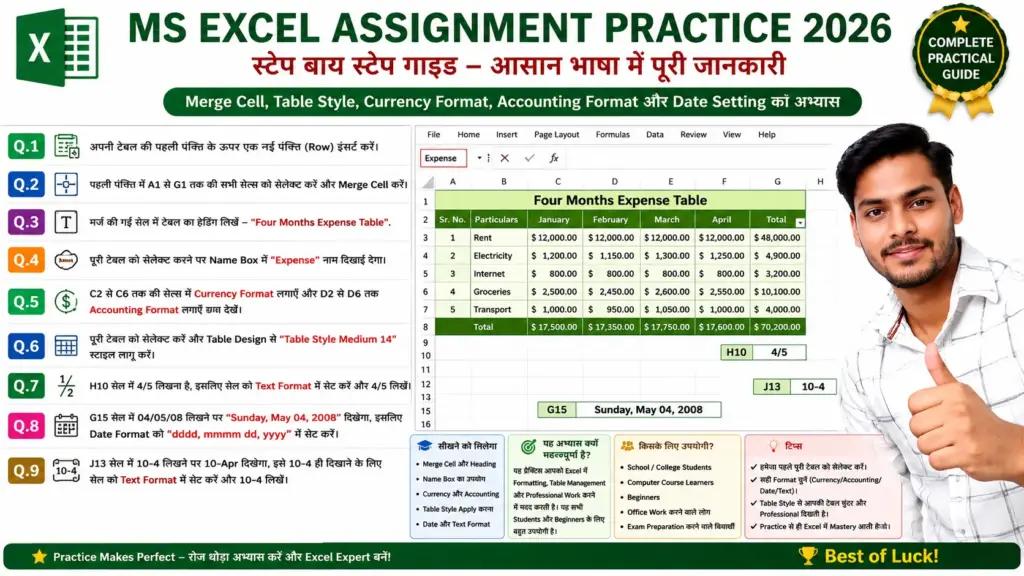
Excel Assignment Practical 03: जानिए Merge Cell, Name Box और Table Formatting का सही तरीका
Q.1- Open your Excel file & insert a row above the first row of your table.
Steps:
- Open your MS Excel file.
- Select the first row of the table.
- Go to the Home tab.
- Click on Insert option.
- Choose Insert Sheet Rows.
- A new row will be inserted above the first row.
Q.2- Now select first row upto seventh columns & apply merge cell.
Steps:
- Select cells from A1 to G1.
- Go to the Home tab.
- Click on Merge & Center option.
- Selected cells will merge into one cell.
Q.3- Give table heading as “Four Months Expense Table”.
Steps:
- Click on the merged cell.
- Type: Four Months Expense Table
- Press Enter key.
Q.4- When you select the entire table Expense will be displayed in the Name Box.
Steps:
- Select the complete table.
- Click inside the Name Box (left side of Formula Bar).
- Type the name Expense.
- Press Enter key.
Q.5- Select the cell from C2 to C6, apply Currency format & from D2 to D6 apply Accounting format, see the effect.
Steps:
- Select cells C2 to C6.
- Go to Home → Number Group.
- Select Currency Format.
- Now select cells D2 to D6.
- Apply Accounting Format.
- Observe the difference between both formats.
Q.6- Select your table and apply table format as “Table Style Medium 14”.
Steps:
- Select the complete table.
- Go to the Home tab.
- Click on Format as Table.
- Choose Table Style Medium 14.
- Click OK.
Q.7- In the cell H10 you want to write the given number 4/5, so do the appropriate setting.
Steps:
- Select cell H10.
- Right click and choose Format Cells.
- Select Text category.
- Click OK.
- Now type 4/5.
- Excel will display it exactly as entered.
Q.8- In the cell G15 when you write 04/05/08 it will show Sunday, May 04, 2008.
Steps:
- Select cell G15.
- Right click and choose Format Cells.
- Select Date category or Custom Format.
- Use the format:
dddd, mmmm dd, yyyy - Click OK.
- Type 04/05/08.
- Output will display as Sunday, May 04, 2008.
Q.9- In the cell J13 when you write 10-4 it will display 10-Apr, but you want to see 10-4 so apply the appropriate setting.
Steps:
- Select cell J13.
- Right click and choose Format Cells.
- Select Text category.
- Click OK.
- Now type 10-4.
- Excel will display exactly 10-4 instead of 10-Apr.